机器学习总结

0、概述

    这段时间主要学习了kaggle网站上的“机器学习”的部分。之前很长一段时间都是在学习
理论,没有机会实践,Kaggle是个不错的平台,有很多使用的难题等待着全世界聪敏的头脑
去解决。通过本篇的学习,很好的将理论知识用到了实践当中,比如之前学习到的绘制模型在
样本集和测试集上的准确率,防止模型过拟合和欠拟合,选择最优的点。还有之前不明白交叉
验证的作用,以及实际效果。网址:https://www.kaggle.com/learn/machine-learning
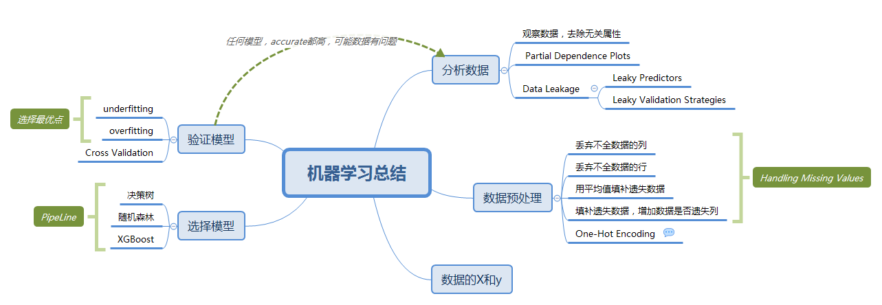
1、思维导图

机器学习总结

2、步骤

2.1、分析数据

1
2
3
4
5
6
7
8
9
10
11
12
13
14
15
16
17
18
19
20
21
22
23
24
25
26
27
28
29
30
31
32
33
34
35
36
37
38
39
40
41
42
43
44
45
46
47
48
49
50
51
52
53
54
############## 观察数据 ##############
import pandas as pd
# save filepath to variable for easier access
melbourne_file_path = '../input/melbourne-housing-snapshot/melb_data.csv'
# read the data and store data in DataFrame titled melbourne_data
melbourne_data = pd.read_csv(melbourne_file_path)
# print a summary of the data in Melbourne data
print(melbourne_data.describe())
print(melbourne_data.columns)

############## 选择过滤数据 ##############
# store the series of prices separately as melbourne_price_data.
melbourne_price_data = melbourne_data.Price
# the head command returns the top few lines of data.
print(melbourne_price_data.head())
columns_of_interest = ['Landsize', 'BuildingArea']
two_columns_of_data = melbourne_data[columns_of_interest]
two_columns_of_data.describe()

y = melbourne_data.Price
melbourne_predictors = ['Rooms', 'Bathroom', 'Landsize', 'Lattitude', 'Longtitude']
X = melbourne_data[melbourne_predictors]

############## Partial Dependence Plots ##############
import pandas as pd
from sklearn.ensemble import GradientBoostingRegressor, GradientBoostingClassifier
from sklearn.ensemble.partial_dependence import partial_dependence, plot_partial_dependence
from sklearn.preprocessing import Imputer

cols_to_use = ['Distance', 'Landsize', 'BuildingArea']

def get_some_data():
data = pd.read_csv('../input/melbourne-housing-snapshot/melb_data.csv')
y = data.Price
X = data[cols_to_use]
my_imputer = Imputer()
imputed_X = my_imputer.fit_transform(X)
return imputed_X, y


X, y = get_some_data()
my_model = GradientBoostingRegressor()
my_model.fit(X, y)
my_plots = plot_partial_dependence(my_model,
features=[0,2],
X=X,
feature_names=cols_to_use,
grid_resolution=10)

############## Data Leakage ##############
# Leaky Predictors
# 数据集中包含预测时不可用的数据。比如,患有癌症的病人,使用了抗生素。
# Leaky Validation Strategy
# 检验策略有问题。或者测试集的数据影响了验证集数据。比如,调用train_test_split之前运行预处理(如为缺失值拟合Imputer)。

Data_Leakage

2.2、数据处理

1
2
3
4
5
6
7
8
9
10
11
12
13
14
15
16
17
18
19
20
21
22
23
24
25
26
27
28
29
30
31
32
33
34
35
36
37
38
39
40
41
42
43
44
45
46
47
48
49
50
51
52
53
54
55
56
57
58
59
60
61
62
63
64
65
66
67
68
69
70
71
72
73
74
75
76
77
78
79
80
81
82
83
84
85
86
87
88
89
90
91
92
93
94
95
96
97
############## 检查数据是否有空项 ##############
print(data.isnull().sum())

############## 丢掉含有空的数据列 ##############
cols_with_missing = [col for col in X_train.columns
if X_train[col].isnull().any()]
reduced_X_train = X_train.drop(cols_with_missing, axis=1)
reduced_X_test = X_test.drop(cols_with_missing, axis=1)
print("Mean Absolute Error from dropping columns with Missing Values:")
print(score_dataset(reduced_X_train, reduced_X_test, y_train, y_test))

############## 填充空的数据列 ##############
from sklearn.preprocessing import Imputer

my_imputer = Imputer()
imputed_X_train = my_imputer.fit_transform(X_train)
imputed_X_test = my_imputer.transform(X_test)
print("Mean Absolute Error from Imputation:")
print(score_dataset(imputed_X_train, imputed_X_test, y_train, y_test))

############## 扩展填充空的数据列 ##############
imputed_X_train_plus = X_train.copy()
imputed_X_test_plus = X_test.copy()

cols_with_missing = (col for col in X_train.columns
if X_train[col].isnull().any())
for col in cols_with_missing:
imputed_X_train_plus[col + '_was_missing'] = imputed_X_train_plus[col].isnull()
imputed_X_test_plus[col + '_was_missing'] = imputed_X_test_plus[col].isnull()

# Imputation
my_imputer = Imputer()
imputed_X_train_plus = my_imputer.fit_transform(imputed_X_train_plus)
imputed_X_test_plus = my_imputer.transform(imputed_X_test_plus)

print("Mean Absolute Error from Imputation while Track What Was Imputed:")
print(score_dataset(imputed_X_train_plus, imputed_X_test_plus, y_train, y_test))

############## 将非数值列One-Hot Encoding ##############
# Read the data
import pandas as pd
train_data = pd.read_csv('../input/train.csv')
test_data = pd.read_csv('../input/test.csv')

# Drop houses where the target is missing
train_data.dropna(axis=0, subset=['SalePrice'], inplace=True)

target = train_data.SalePrice

# Since missing values isn't the focus of this tutorial, we use the simplest
# possible approach, which drops these columns.
# For more detail (and a better approach) to missing values, see
# https://www.kaggle.com/dansbecker/handling-missing-values
cols_with_missing = [col for col in train_data.columns
if train_data[col].isnull().any()]
candidate_train_predictors = train_data.drop(['Id', 'SalePrice'] + cols_with_missing, axis=1)
candidate_test_predictors = test_data.drop(['Id'] + cols_with_missing, axis=1)

# "cardinality" means the number of unique values in a column.
# We use it as our only way to select categorical columns here. This is convenient, though
# a little arbitrary.
low_cardinality_cols = [cname for cname in candidate_train_predictors.columns if
candidate_train_predictors[cname].nunique() < 10 and
candidate_train_predictors[cname].dtype == "object"]
numeric_cols = [cname for cname in candidate_train_predictors.columns if
candidate_train_predictors[cname].dtype in ['int64', 'float64']]
my_cols = low_cardinality_cols + numeric_cols
train_predictors = candidate_train_predictors[my_cols]
test_predictors = candidate_test_predictors[my_cols]

print(train_predictors.dtypes.sample(10))

one_hot_encoded_training_predictors = pd.get_dummies(train_predictors)
from sklearn.model_selection import cross_val_score
from sklearn.ensemble import RandomForestRegressor

def get_mae(X, y):
# multiple by -1 to make positive MAE score instead of neg value returned as sklearn convention
return -1 * cross_val_score(RandomForestRegressor(50),
X, y,
scoring = 'neg_mean_absolute_error').mean()

predictors_without_categoricals = train_predictors.select_dtypes(exclude=['object'])

mae_without_categoricals = get_mae(predictors_without_categoricals, target)

mae_one_hot_encoded = get_mae(one_hot_encoded_training_predictors, target)

print('Mean Absolute Error when Dropping Categoricals: ' + str(int(mae_without_categoricals)))
print('Mean Abslute Error with One-Hot Encoding: ' + str(int(mae_one_hot_encoded)))

############## 多个文件join ##############
one_hot_encoded_training_predictors = pd.get_dummies(train_predictors)
one_hot_encoded_test_predictors = pd.get_dummies(test_predictors)
final_train, final_test = one_hot_encoded_training_predictors.align(one_hot_encoded_test_predictors,
join='left',
axis=1)

2.3、选择模型

1
2
3
4
5
6
7
8
9
10
11
12
13
14
15
16
17
18
19
20
21
22
23
24
25
26
27
28
29
30
31
32
33
34
35
36
37
38
############## 决策树回归 ##############
from sklearn.tree import DecisionTreeRegressor

# Define model
melbourne_model = DecisionTreeRegressor()

# Fit model
melbourne_model.fit(X, y)

print("Making predictions for the following 5 houses:")
print(X.head())
print("The predictions are")
print(melbourne_model.predict(X.head()))

############## 随机森林 ##############
from sklearn.ensemble import RandomForestRegressor
from sklearn.metrics import mean_absolute_error

forest_model = RandomForestRegressor()
forest_model.fit(train_X, train_y)
melb_preds = forest_model.predict(val_X)
print(mean_absolute_error(val_y, melb_preds))

############## XGBoost ##############
from xgboost import XGBRegressor

my_model = XGBRegressor()
# Add silent=True to avoid printing out updates with each cycle
my_model.fit(train_X, train_y, verbose=False)

############## PipeLines ##############
from sklearn.ensemble import RandomForestRegressor
from sklearn.pipeline import make_pipeline
from sklearn.preprocessing import Imputer

my_pipeline = make_pipeline(Imputer(), RandomForestRegressor())
my_pipeline.fit(train_X, train_y)
predictions = my_pipeline.predict(test_X)

2.4、验证模型

1
2
3
4
5
6
7
8
9
10
11
12
13
14
15
16
17
18
19
20
21
22
23
24
25
26
27
28
29
30
31
32
33
34
35
36
37
38
39
40
41
42
43
44
45
46
47
48
49
50
51
52
53
54
55
56
57
58
59
60
61
62
63
64
65
66
67
68
############## 模型在测试集上的误差 ##############
from sklearn.model_selection import train_test_split

# split data into training and validation data, for both predictors and target
# The split is based on a random number generator. Supplying a numeric value to
# the random_state argument guarantees we get the same split every time we
# run this script.
train_X, val_X, train_y, val_y = train_test_split(X, y,random_state = 0)
# Define model
melbourne_model = DecisionTreeRegressor()
# Fit model
melbourne_model.fit(train_X, train_y)

# get predicted prices on validation data
val_predictions = melbourne_model.predict(val_X)
print(mean_absolute_error(val_y, val_predictions))

############## 绘制不同个数叶子节点的误差 ##############
from sklearn.metrics import mean_absolute_error
from sklearn.tree import DecisionTreeRegressor

def get_mae(max_leaf_nodes, predictors_train, predictors_val, targ_train, targ_val):
model = DecisionTreeRegressor(max_leaf_nodes=max_leaf_nodes, random_state=0)
model.fit(predictors_train, targ_train)
preds_val = model.predict(predictors_val)
mae = mean_absolute_error(targ_val, preds_val)
return(mae)

# Data Loading Code Runs At This Point
import pandas as pd

# Load data
melbourne_file_path = '../input/melbourne-housing-snapshot/melb_data.csv'
melbourne_data = pd.read_csv(melbourne_file_path)
# Filter rows with missing values
filtered_melbourne_data = melbourne_data.dropna(axis=0)
# Choose target and predictors
y = filtered_melbourne_data.Price
melbourne_predictors = ['Rooms', 'Bathroom', 'Landsize', 'BuildingArea',
'YearBuilt', 'Lattitude', 'Longtitude']
X = filtered_melbourne_data[melbourne_predictors]

from sklearn.model_selection import train_test_split

# split data into training and validation data, for both predictors and target
train_X, val_X, train_y, val_y = train_test_split(X, y,random_state = 0)

# compare MAE with differing values of max_leaf_nodes
plot_x = []
plot_y = []
for max_leaf_nodes in np.arange(10,1000,5):
my_mae = get_mae(max_leaf_nodes, train_X, test_X, train_y, test_y)
print("Max leaf nodes: %d \t\t Mean Absolute Error: %d" %(max_leaf_nodes, my_mae))
plot_x.append(max_leaf_nodes)
plot_y.append(my_mae)

plt.plot(plot_x, plot_y)
print("index:%f,nodes:%f"%(plot_y.index(min(plot_y)),plot_x[plot_y.index(min(plot_y))]))
plt.show()

############## Cross Validation ##############
from sklearn.ensemble import RandomForestRegressor
from sklearn.pipeline import make_pipeline
from sklearn.preprocessing import Imputer
my_pipeline = make_pipeline(Imputer(), RandomForestRegressor())
from sklearn.model_selection import cross_val_score
scores = cross_val_score(my_pipeline, X, y, scoring='neg_mean_absolute_error')
print('Mean Absolute Error %2f' %(-1 * scores.mean()))

3、总结

机器学习是一种数据处理的科学,采用科学的分析方式调整模型的参数,试验的数据,达到提高识别率的目的。
坚持原创技术分享,您的支持将鼓励我继续创作!